Aligning recordings from independent sensors

Luna's INSERT command exists for a practical reason: independent recording systems rarely agree perfectly about time. This can make aligning concurrently recorded signals -- for example, from a wearable and a traditional PSG performed on the same night -- difficult.

To illustrate some of these issues, here we use a real example from Nox and X-trodes recordings of the same subject on the same night. The Nox EDF starts at 22:00:01 and the X-trodes EDF starts at 22:26:09: that is, the EDF headers alone imply a start offset of just over 26 minutes (1,568 seconds) that must be accounted for. We merged the two recordings to make a single EDF, assuming the two original EDF header times were accurate (using the INSERT command, as shown below).

Here's header information for the Nox recording:

luna nox.edf -s DESC

 duration 10.00.30, 36030s | time 22.00.01 - 08.00.31 | date 17.07.23

and for X-trodes:

luna xtrodes.edf -s DESC

 duration 08.56.40, 32200s | time 22.26.09 - 07.22.49 | date 17.07.23

We'll initially compare the two frontal channels (F3-M2 and F4-M1) from the Nox device with the two frontal X-trodes channels (approximately positioned near AF3/Fp1 and AF4/Fp2). A cursory visual review of the signals (using Lunascope) shows nontrivial issues in aligning these two recordings.

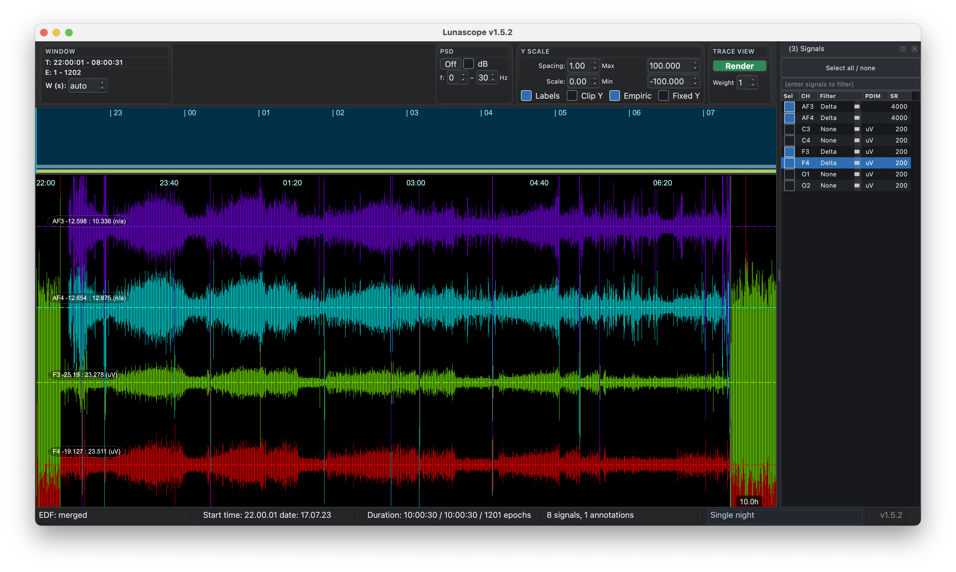
At a broad, zoomed-out level we see the expected correspondence between devices: the two Nox frontal channels are shown in the lower two traces, and the two X-trodes channels are shown in the top two traces. Here, we've delta-band filtered the signals to highlight the ultradian variation in slow wave sleep over the night, making their correspondence clearer (note that the high-amplitude noise at the start/end of the Nox recording, while X-trodes was not recording, likely reflects movement during the pre-lights out period):

However, zooming in we see a clear divergence in the signals around 23:05:22, early in the recording, even after adjusting for the different start times (as per the EDF headers). Naturally these are different channels and are not expected to align completely, but visual review around this area makes the relative timing of the signals quite clear. (Open the picture in a separate tab to zoom in and see it more clearly.)

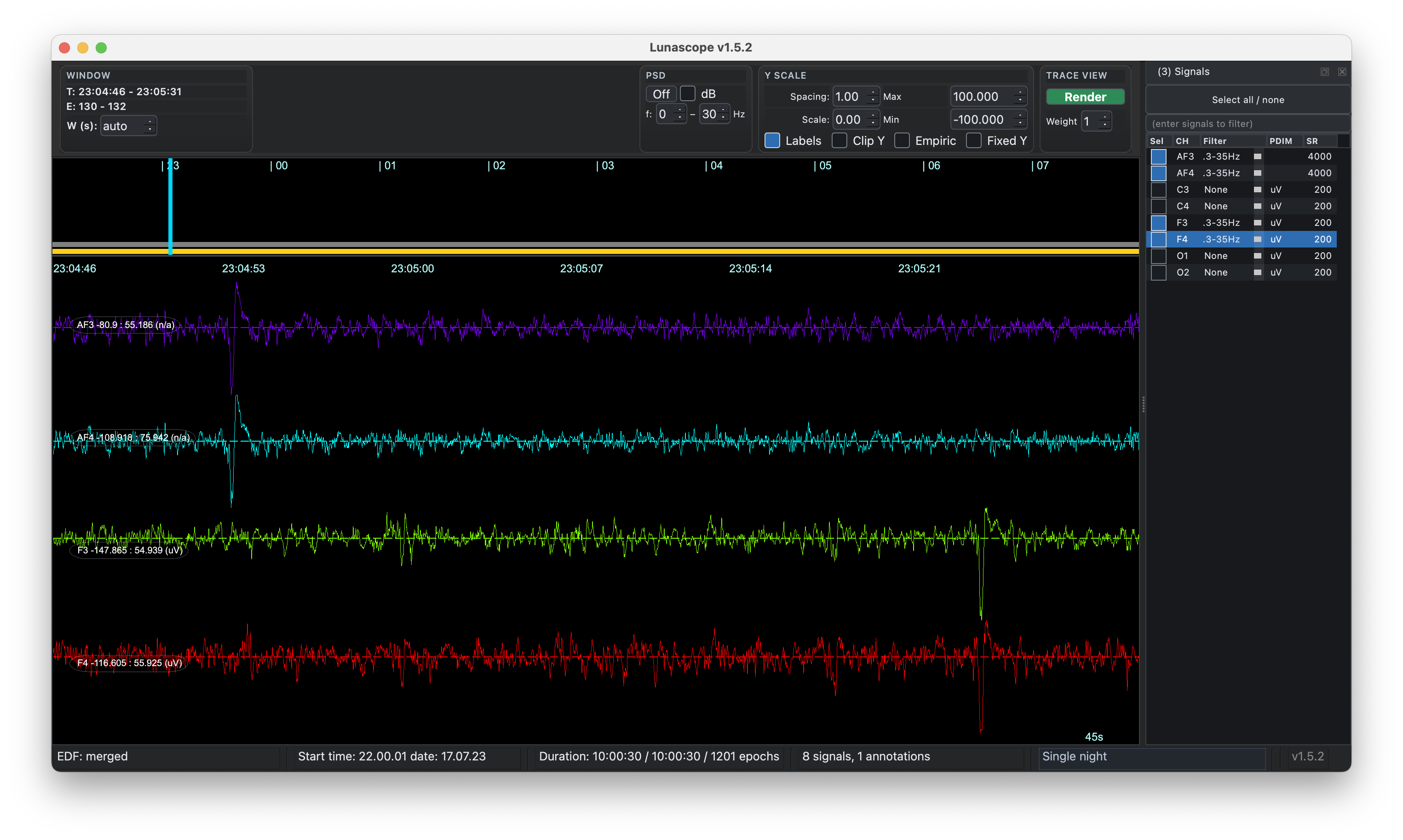
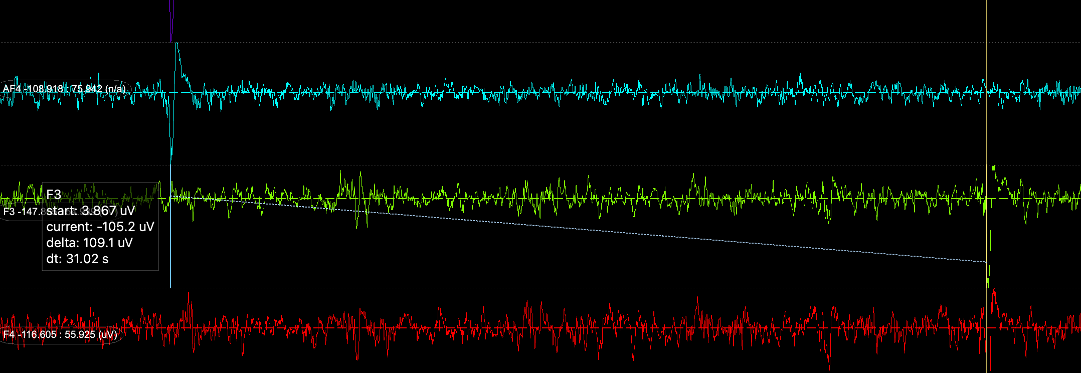
In this case, there is a difference of approximately 31.0 seconds - even after correcting for the EDF header start times - with the X-trodes signals coming earlier than expected, relative to the Nox. Here we measure the time difference with Lunascope's probe option:

This might simply suggest that one (or both) of the clocks was not properly synchronized, and so the times in the EDF header are not fully accurate. Naturally this is important to note and correct in any case - but further review suggests something else going on between these recordings. When looking at other clear 'landmark' points later in the night, we find the gap has shrunk - and by quite a lot. Here at 04:26:16, the gap is almost 8 seconds shorter, with only 23.1 seconds between points.

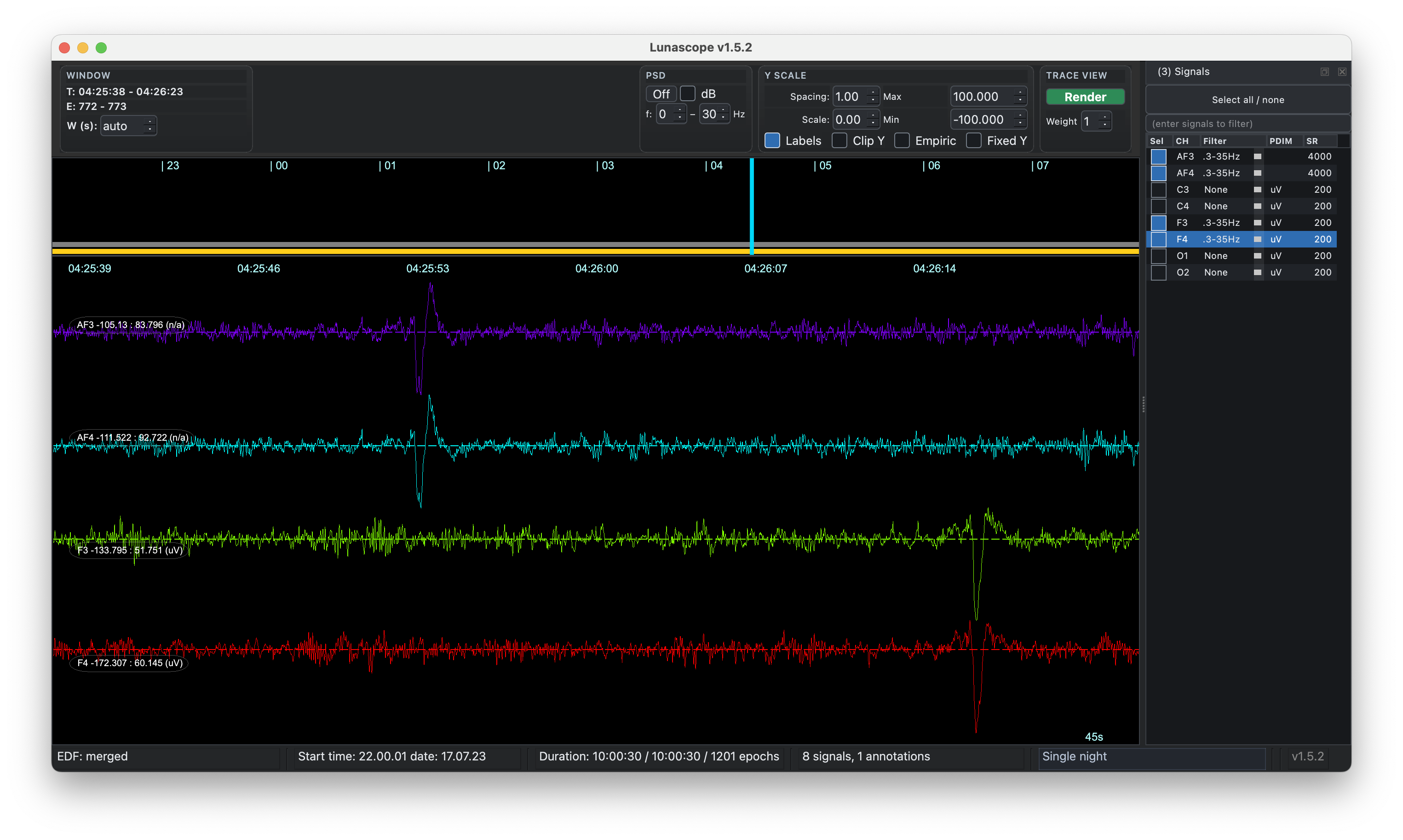
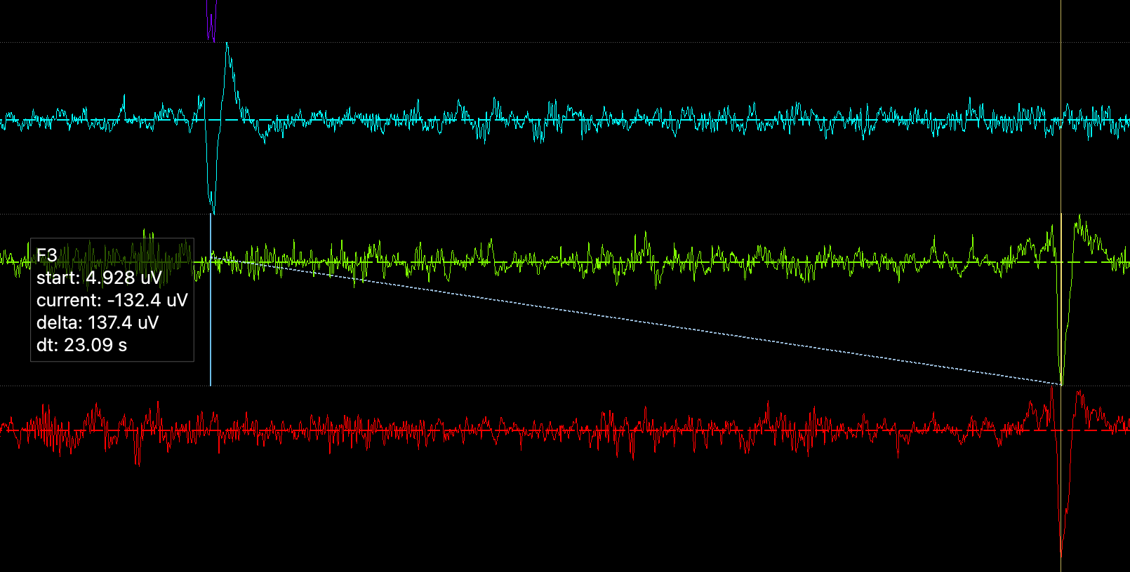
This change of almost 8 seconds over a period of almost 20,000 seconds (from 11pm to 4:30am) corresponds to a drift rate between clocks of 0.04% - around 400 ppm. If this reflected a continuous drift due to different effective sampling rates, this would imply the nominal rate of 200 Hz is more like 200.08 Hz for X-trodes (here assuming the Nox device is exactly 200 Hz, although of course from this comparison alone we can only determine a difference; we cannot make absolute statements about which device is the more accurate).

---

This preliminary visual review begs several questions:

• are the EDF header clocks really not well specified?

• is there a continuous drift between device clocks?

• or was there perhaps a gap in recording for one of the devices that occurred between these two time points?

• how do we fix this?

This is the motivation for the INSERT command.

Sources of misalignment

In general, there are several potential sources of discrepancy between EDF-based recordings:

• standard EDF headers only encode start time to 1 second resolution
• unsynchronized clocks
• manual header edits or offsets
• unannotated gaps or pauses in recording
• nominal sample rates that are not quite the true sample rates

Considering this last issue: whereas two devices may have nominal sampling rates of 200 Hz, in practice they may vary by small amounts - both between each other and within themselves over time. The stability of a quartz oscillator clock can vary depending on factors such as temperature, the age of the crystal, mechanical stress, humidity, power supply voltage, magnetic fields, and so on. Most consumer or mid-grade electronic devices likely have quartz oscillators that have a tolerance around 10 - 50 ppm (parts per million) or worse. For a signal sampled at 200 Hz, this might correspond to an error around 0.01 Hz.

On top of the quartz oscillator, analog-to-digital converters (ADC) and other factors may impose further discrepancies, further compounding differences between devices. Especially in wearables, sampling may be triggered by software-specific factors such as interrupts, the OS scheduler, buffer filling, etc., which may introduce jitter and occasionally dropped or duplicated samples. Suboptimal anti-aliasing/digital filtering or data transmission artifacts can further degrade the accuracy and stability of the true sampling rate.

Over long recordings, tiny timing mismatches can become visible if they accumulate, meaning that the two clocks will appear to systematically and continuously drift relative to each other. Practically, for most analyses this will likely not matter. However, when comparing or merging signals across different sensors, such effects can matter a great deal: a few seconds of drift can completely stop channels from lining up. Depending on the scale of drift and the nature of the recording, attempts to align EEG transients (e.g. spindles) will be impacted, and possibly even epoch-level comparisons too.

INSERT command

Rather than trusting a single header timestamp, the INSERT command is designed to align two EDFs empirically, and merge them in a way that adjusts for certain types of timing artifact. Specifically, it:

1. takes a set of similar signal pairs across the two EDFs

2. estimates the best local lag in many windows by cross-correlation

3. fits the linear change in lag over time

4. optionally, uses that fitted offset plus drift to insert the secondary signal on the primary EDF timeline

Even when there is no real timing problem to correct, INSERT can still be a useful way to merge EDFs. It supports sub-second fractional alignment, allows the inserted signals to have different sample rates from the reference EDF, and can handle recordings that only partially overlap in time; where inserted signals extend into uncovered regions, those gaps are zero-padded. One practical consequence is that the output is always defined on the reference EDF timeline, and so has the same duration as the reference EDF. In that sense, the operation is asymmetric: one EDF is the timeline anchor, and the other is inserted into it.

Simulated data examples

Before applying INSERT to real data, let's first apply it to data where we know the ground truth by design. We'll extract only the O1-M2 channel from the Nox device and then create several copies that introduce different types of timing differences:

1. an exact copy, perfectly aligned

2. a version that is filtered - and so no longer digitally identical - but is still aligned in time with itself (n.b. all subsequent copies are based on this filtered copy too)

3. a version where we introduce an offset between the two signals (by misspecifying the start time)

4. a version where we introduce a drift between the two signals (by misspecifying the sample rate for one)

5. a version with a multi-second region spliced out - so that one signal drops some data but would appear to jump ahead relative to the other original

6. a version with all the above: a time offset, a gap/jump and a drift

Self comparisons

We start by extracting the O1-M2 channel from nox.edf and saving a new reference EDF r0.edf, renamed to just O1 (although we could have just used the original nox.edf in these examples):

luna nox.edf sig=O1 -s WRITE edf=r0 

We create an identical version by simply copying the file r0.edf to r-copy.edf (although we could have just used r0.edf twice in the example below too).

We run INSERT specifying the comparison edf and the pairs of channels used (here, both O1):

luna r0.edf -o out.db -s INSERT edf=r-copy.edf pairs=O1,O1 

  header-derived offset: -0 seconds (negative = edf2 starts after edf1)
  using header-derived offset-range: -60 to 60 seconds
  method: xcorr, bandpass 0.5-15 Hz;  300s windows every 60s,  range 3603-32427s

  summary across 481 window(s):
    quality          accepted=481/481 (100%)  peak median=1  mean=1  min=1  max=1
    waveform_shift   median=0s  mean=0s  p10=0s  p90=0s  min=0s  max=0s  range=0s
    fit_shift        used=481/481  median=0s  mean=0s  p10=0s  p90=0s  min=0s  max=0s  range=0s
    offset           -0s (start_shift=0s, header_offset=-0s)
    drift            slope=0 s/s  (0 s/hr)  intercept=0s  R2=1
    implied SR of secondary: 200 Hz  (nominal: 200 Hz)
    (positive slope = secondary clock running faster than primary)
  per-pair drift:
    O1..O1:  slope=0 s/s (0 s/hr)  intercept=0s  implied SR=200 Hz

As noted in the console log, by default INSERT looks at 300s windows spaced one minute apart across most of the night (skipping periods near the start and end, which tend to be artifact-ridden, and are more likely to not have a matching partner in the other recording, if recordings were of different durations).

Based on the cross-correlation between signals, this analysis correctly suggests that there is no drift or offset between the recordings - all windows have a perfect cross correlation (under the quality line) with an implied offset of 0s. That is, when similar signals truly align, this command correctly suggests that.

Filtered data

Next, we'll make a filtered (2 - 20 Hz) copy of the signal and save it as r-flt.edf:

luna r0.edf -s ' FILTER bandpass=2,20 tw=2 ripple=0.01 & WRITE edf=r-flt '

Re-running INSERT between r0.edf and r-flt.edf:

  header-derived offset: -0 seconds (negative = edf2 starts after edf1)
  using header-derived offset-range: -60 to 60 seconds
  method: xcorr, bandpass 0.5-15 Hz;  300s windows every 60s,  range 3603-32427s
  summary across 437 window(s):
    quality          accepted=437/481 (90.8524%)  peak median=0.75  mean=0.67  min=0.20  max=0.92
    waveform_shift   median=0s  mean=0s  p10=0s  p90=0s  min=0s  max=0s  range=0s
    fit_shift        used=437/437  median=0s  mean=0s  p10=0s  p90=0s  min=0s  max=0s  range=0s
    offset           -0s (start_shift=0s, header_offset=-0s)
    drift            slope=0 s/s  (0 s/hr)  intercept=0s  R2=1
    implied SR of secondary: 200 Hz  (nominal: 200 Hz)
    (positive slope = secondary clock running faster than primary)
  per-pair drift:
    O1..O1:  slope=0 s/s (0 s/hr)  intercept=0s  implied SR=200 Hz

We now see that the cross-correlations vary between 0.2 and 0.9, reflecting the impact of filtering. Correspondingly, some windows were deemed not to have sufficiently high cross correlations to accurately determine their offset - here, almost 10% of windows were dropped (under the quality row). However, across every retained window the offset is still exactly 0s, correctly implying that there is no drift or offset between these signals.

For illustration, we can push this a step further such that we'd expect the correspondence of the two signals to break down - here we arbitrarily impose a very strict (30-31 Hz) filter, essentially removing almost all of the physiological variation in this copy:

luna r0.edf -s 'FILTER bandpass=30,31 tw=2 ripple=0.01 & WRITE edf=r-flt '

Re-running INSERT with this noise comparison, we now see a different pattern:

  header-derived offset: -0 seconds (negative = edf2 starts after edf1)
  using header-derived offset-range: -60 to 60 seconds
  method: xcorr, bandpass 0.5-15 Hz;  300s windows every 60s,  range 3603-32427s
  summary across 481 window(s):
    quality          accepted=481/481 (100%)  peak median=0.708022  mean=0.711173  min=0.59971  max=0.964224
    waveform_shift   median=0.565s  mean=0.0135031s  p10=-0.565s  p90=0.565s  min=-0.57s  max=0.575s  range=1.145s
    fit_shift        used=481/481  median=0.565s  mean=0.0135031s  p10=-0.565s  p90=0.565s  min=-0.57s  max=0.575s  range=1.145s
    offset           0.0221875s (start_shift=-0.0221875s, header_offset=-0s)
    drift            slope=1.98248e-06 s/s  (0.00713694 s/hr)  intercept=-0.0221875s  R2=0.00085602
    implied SR of secondary: 200 Hz  (nominal: 200 Hz)
    (positive slope = secondary clock running faster than primary)
  warning: alignment quality may be poor: R2=0.00085602 < 0.5
  hints:
    - try a smaller len window (current len=300s)
    - use offset-margin to search around the header-derived offset (current default margin=60s; effective range=-60 to 60s)
    - set an absolute offset-range around the expected shift (current offset-range=unset; effective range=-60 to 60s)
    - use full-search when EDF start times are missing or not trusted (current full-search=no)
    - add verbose=1 to diagnose per-window results (current verbose=no)
  per-pair drift:
    O1..O1:  slope=1.98248e-06 s/s (0.00713694 s/hr)  intercept=-0.0221875s  implied SR=200 Hz

Of note:

• all windows met the default criteria for showing a sufficient correlation

• however -- and most significantly -- the drift estimate R2 (which also tracks the consistency of the offset estimates) is effectively zero

• because of this, we see a warning is issued (warning: alignment quality may be poor)

It is possible for this type of message to reflect two recordings that are extremely misaligned (e.g. with an offset of tens of minutes), meaning that the default windowing strategy missed them (this is why the warning also gives hints about extending the search space to capture search issues).

However -- as in this example -- this can also reflect that the pairs of signals used to align the data are fundamentally too different and so cannot be meaningfully aligned. If this is the case, then not much can be done except to use different signals if they are available, or to post-process both signals to be more comparable.

Bottom line: INSERT is agnostic to the type of signals used (they do not have to be EEGs, for example), but it is premised on the signals a) showing meaningful variability over the night, and b) being roughly similar across the two recordings.

Offset

Next, using the "lightly" filtered copy from the last section, we'll create a timing offset between the two recordings, by changing only the EDF header start time for the second EDF, advancing it from 22.00.01 by 12 seconds:

luna r-flt.edf -s ' SET-HEADERS start-time=22.00.13 & WRITE edf=r-offset '

Re-running INSERT:

luna r0.edf -o out.db -s ' INSERT edf=r-offset.edf pairs=O1,O1 '

  header-derived offset: -12 seconds (negative = edf2 starts after edf1)
  using header-derived offset-range: -72 to 48 seconds
  method: xcorr, bandpass 0.5-15 Hz;  300s windows every 60s,  range 3603-32427s
  summary across 437 window(s):
    quality          accepted=437/481 (90.9%)  peak median=0.76  mean=0.67  min=0.20  max=0.92
    waveform_shift   median=0s  mean=0s  p10=0s  p90=0s  min=0s  max=0s  range=0s
    fit_shift        used=437/437  median=0s  mean=0s  p10=0s  p90=0s  min=0s  max=0s  range=0s
    offset           -12s (start_shift=0s, header_offset=-12s)
    drift            slope=0 s/s  (0 s/hr)  intercept=0s  R2=1
    implied SR of secondary: 200 Hz  (nominal: 200 Hz)
    (positive slope = secondary clock running faster than primary)
  per-pair drift:
    O1..O1:  slope=0 s/s (0 s/hr)  intercept=0s  implied SR=200 Hz

We now see the offset of -12 seconds, correctly inferred from the EDF headers. (The offset is negative, as it reflects the correction to add to the secondary timeline to align it to the primary one.)

The waveform_shift values are derived from the cross correlation analyses, meaning that after adjusting for the header difference, no further waveform shifts are necessary. To illustrate these different effects, consider another offset example:

luna r-flt.edf -s ' SET-HEADERS start-time=22.01.00
                    MASK mask-epoch=1 & RE
                    WRITE edf=r-offset '

That is, the EDF header is shifted now 59 seconds forward (from 22.00.01 to 22.01.00) but we also chop off the first epoch. Luna's WRITE will adjust the EDF header time by a further +30 seconds to account for this - so r-offset.edf will have a final start time of 22.01.30, but will actually start at 22.00.31, i.e. the true time (based on the original signal) for the start of the second epoch.

Now re-running INSERT:

  header-derived offset: -89 seconds (negative = edf2 starts after edf1)
  using header-derived offset-range: -149 to -29 seconds
  method: xcorr, bandpass 0.5-15 Hz;  300s windows every 60s,  range 3600-32400s
  summary across 436 window(s):
    quality          accepted=436/481 (90.6%)  peak median=0.76  mean=0.68  min=0.20  max=0.92
    waveform_shift   median=-30s  mean=-30s  p10=-30s  p90=-30s  min=-30s  max=-30s  range=0s
    fit_shift        used=436/436  median=-30s  mean=-30s  p10=-30s  p90=-30s  min=-30s  max=-30s  range=0s
    offset           -59s (start_shift=-30s, header_offset=-89s)
    drift            slope=0 s/s  (0 s/hr)  intercept=-30s  R2=1
    implied SR of secondary: 200 Hz  (nominal: 200 Hz)
    (positive slope = secondary clock running faster than primary)
  per-pair drift:
    O1..O1:  slope=0 s/s (0 s/hr)  intercept=-30s  implied SR=200 Hz

We see the apparent 89s header offset has been corrected by -30s, resulting in the final, correct -59s offset. If you trust INSERT you don't need to look at these outputs in too much detail, but briefly:

• header_offset is the known timing difference from the EDF start times alone

• waveform_shift is the additional correction still needed after accounting for that header difference, estimated from the signals themselves by cross-correlation

• fit_shift is similar to waveform_shift but based only on the subset of accepted windows that are not rejected by outlier removal at the drift fit step (controlled by fit-outlier-sd and fit-outlier-passes, by default 3 SD and 2 passes); here it is identical to waveform_shift

• offset is the net timing correction (these two previous offsets combined) that must be applied to the secondary recording to align it to the primary. Negative means shift the secondary earlier; positive means shift it later

Drift

Next, we create drift in one of the signals, by misspecifying the true sampling rate. We take the filtered 200 Hz signal, resample it to 200.1 Hz and then save it as a text file (s.txt, which has just one numeric value per row):

luna r-flt.edf -s ' RESAMPLE sr=200.1 & MATRIX file=s.txt min '

Next we create an EDF from this sample but specify a nominal rate of exactly 200 Hz when reading it in:

luna s.txt --fs=200 --time=22.00.01 --date=17.07.23 --chs=O1 -s WRITE edf=r-drift

This trick (using an intermediate text representation of the signal that, unlike EDF, loses explicit information about sampling rate) lets us effectively mimic a clock that is "too fast" here. Note that we specify the start time/date to match the original - i.e. there is no further offset here, just clock drift. This is a 0.05% (500 ppm) drift effect, which is relatively large, leading to a drift of almost 15 seconds over an 8 hour recording.

We now run INSERT on r-drift.edf - i.e. the file that has a signal labelled as 200 Hz but it is in fact 200.1 Hz. Using the default invocation we actually hit a warning:

luna r0.edf -o out.db -s ' INSERT edf=r-drift.edf pairs=O1,O1 '

  header-derived offset: -0 seconds (negative = edf2 starts after edf1)
  using header-derived offset-range: -60 to 60 seconds
  method: xcorr, bandpass 0.5-15 Hz;  300s windows every 60s,  range 3601.8-32416.2s
  summary across 4 window(s):
    quality          accepted=4/481 (0.831601%)  peak median=0.19  mean=0.19  min=0.066  max=0.33
    waveform_shift   median=-16.15s  mean=-17.8s  p10=-19.6s  p90=-15.87s  min=-19.65s  max=-15.75s  range=3.89s
    fit_shift        used=4/4  median=-16.15s  mean=-17.78s  p10=-19.6s  p90=-15.87s  min=-19.65s  max=-15.75s  range=3.89s
    offset           29.8517s (start_shift=-29.8517s, header_offset=-0s)
    drift            slope=0.000495468 s/s  (1.78369 s/hr)  intercept=-29.8517s  R2=0.999822
    implied SR of secondary: 200.099 Hz  (nominal: 200 Hz)
    (positive slope = secondary clock running faster than primary)
  warning: alignment quality may be poor: P_OK=0.00831601 < 0.5; median peak=0.191101 < 0.35
  hints:
    - try a smaller len window (current len=300s)
    - use offset-margin to search around the header-derived offset (current default margin=60s; effective range=-60 to 60s)
    - set an absolute offset-range around the expected shift (current offset-range=unset; effective range=-60 to 60s)
    - use full-search when EDF start times are missing or not trusted (current full-search=no)
    - add verbose=1 to diagnose per-window results (current verbose=no)
  per-pair drift:
    O1..O1:  slope=0.000495468 s/s (1.78369 s/hr)  intercept=-29.8517s  implied SR=200.099 Hz

It closely estimates the slope (reflecting drift implying a sampling rate of 200.099 Hz, instead of true 200.1 Hz), but it only considers 4 valid windows to do this. (Remember this is a simulated example to illustrate the principles behind the approach, in which the second signal is a filtered version of the first; as we'll see, things are less clear-cut in practice.)

The drop out of windows is actually driven by the relatively large simulated drift effect here. That is, at 200.1 Hz, even within a single 300s window (the default unit of the cross correlation analyses) there can be non-negligible drift (0.15s, or 30 samples) which can attenuate cross correlations.

Despite the high R2 for the drift fit, one would rightly be suspicious about an estimate based on only 4 windows. INSERT's behavior can be modified to handle these "low quality" situations better: in this case, a) using a shorter window, b) excluding high-frequency content, as it will be more impacted by drift (by default, INSERT pre-filters signals using a passband of 0.5 - 15 Hz), or c) allowing low-quality windows to contribute to the fit, but being more stringent within outlier removal at the second stage (fitting the linear drift slope), rather than excluding windows up front.

In this example, all of these approaches "fix" the issue. First, we'll just present the results for the first and second combined:

luna r0.edf -o out.db -s ' INSERT edf=r-drift.edf pairs=O1,O1 filt-high=4 len=30 '

  header-derived offset: -0 seconds (negative = edf2 starts after edf1)
  using header-derived offset-range: -60 to 60 seconds
  method: xcorr, bandpass 0.5-4 Hz;  30s windows every 60s,  range 3603-32427s
  summary across 445 window(s) (2 outlier(s) removed from slope fit):
    quality          accepted=445/481 (92.5156%)  peak median=0.574727  mean=0.548914  min=0.172722  max=0.776581
    waveform_shift   median=9.275s  mean=9.07199s  p10=3.137s  p90=14.808s  min=-25.445s  max=16.2s  range=41.645s
    fit_shift        used=443/445  median=9.305s  mean=9.15079s  p10=3.161s  p90=14.814s  min=1.84s  max=16.2s  range=14.36s
    offset           -0.00738022s (start_shift=0.00738022s, header_offset=-0s)
    drift            slope=0.00049 s/s  (1.79 s/hr)  intercept=0.0073s  R2=1
    implied SR of secondary: 200.1 Hz  (nominal: 200 Hz)
    (positive slope = secondary clock running faster than primary)
  per-pair drift:
    O1..O1:  slope=0.00049 s/s (1.79 s/hr)  intercept=0.0073s  implied SR=200.1 Hz  [2 outlier(s) removed]

We now see the vast majority of windows are included, and the estimate of the sample rate is 200.1 Hz exactly. Importantly, the drift line in the console output above shows the R2 of the fit of offset by time over the night is very high (1.0), but is still based on a large number of windows (443). This indicates that the change in offset really does reflect a linear change over the night - i.e. drift. We can see this most clearly by plotting the offsets (and other information) window-by-window. We can extract as a text file (some columns removed for clarity):

destrat out.db +INSERT -r WIN > o.tsv

ID  WIN   DSEC  FIT_OUTLIER   PEAK    T1_HMS     T2_HMS      TOT_SEC
r0  3603  0      -1           0.240   23:00:02   23:00:04    -1.81
r0  3663  0       0           0.303   23:01:02   23:01:04    -1.84
r0  3723  0.03    0           0.395   23:02:02   23:02:04    -1.87
r0  3783  0.06    0           0.559   23:03:02   23:03:04    -1.9
r0  3843  0.09    0           0.703   23:04:02   23:04:04    -1.93
r0  3903  0.12    0           0.719   23:05:02   23:05:04    -1.96
r0  3963  0.145   0           0.737   23:06:02   23:06:04    -1.985
r0  4023  0.18    0           0.744   23:07:01   23:07:04    -2.02
r0  4083  0.21    0           0.679   23:08:01   23:08:04    -2.05
...

Plotting PEAK (Cross correlation) and TOT_SEC (Offset) against window (Time in seconds):

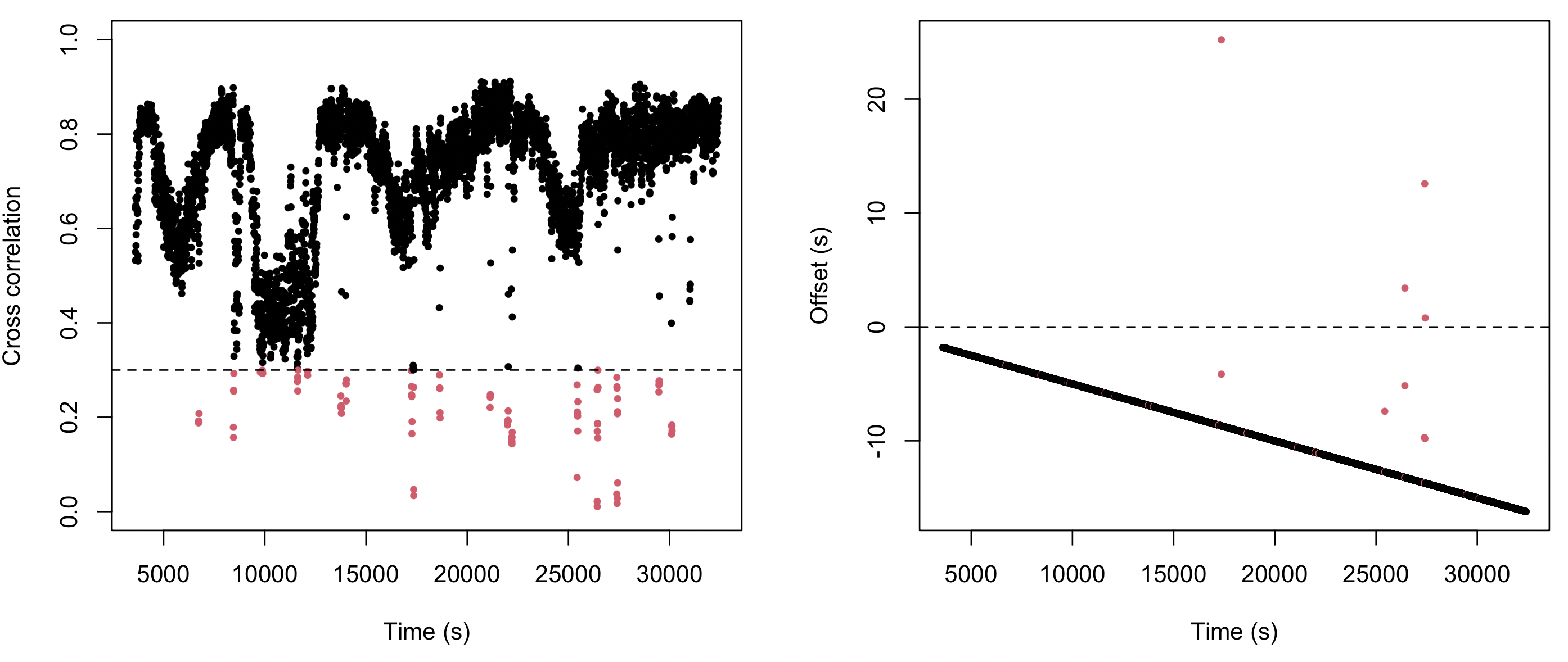
The left panel shows the cross-correlation per window. Those in red are "low quality" and excluded from the drift slope fit. The panel on the right shows the high quality window offset estimates as a function of time; here the red points also include those flagged as outliers in the residual space after regressing on time (this 3SD outlier step is repeated twice). Despite the offsets being independently estimated, there is a very clear - almost perfect - linear trend - which points to linear drift accumulating steadily across the night (as we know to be true in this simulated example). Note that it does not start exactly at 0s offset, as we have excluded the initial (and ending) parts of the recording, given the default value of the start argument.

As noted above, an alternative and complementary approach might instead be to retain the longer, low-quality windows (setting min-peak=0.1 instead of the default of 0.3), but instead be more stringent in the second stage of window exclusion: instead of removing windows based on residuals (after fitting the slope) of 3 SD units (performed twice), we now use a threshold of 2 SD units (repeating this four times):

luna r0.edf -o out.db -s ' INSERT edf=r-drift.edf pairs=O1,O1
                                  min-peak=0.1
                                  fit-outlier-sd=2
                                  fit-outlier-passes=4 '

  header-derived offset: -0 seconds (negative = edf2 starts after edf1)
  using header-derived offset-range: -60 to 60 seconds
  method: xcorr, bandpass 0.5-15 Hz;  300s windows every 60s,  range 3603-32427s
  summary across 471 window(s) (15 outlier(s) removed from slope fit):
    quality          accepted=471/481 (97.9%)  peak median=0.19  mean=0.19  min=0.064  max=0.34
    waveform_shift   median=8.91s  mean=8.98s  p10=3.31s  p90=14.75s  min=1.84s  max=16.29s  range=14.45s
    fit_shift        used=456/471  median=8.79s  mean=8.94s  p10=3.22s  p90=14.76s  min=1.84s  max=16.29s  range=14.45s
    offset           -0.076s (start_shift=0.076s, header_offset=-0s)
    drift            slope=0.00049 s/s  (1.79 s/hr)  intercept=0.076s  R2=0.999
    implied SR of secondary: 200.1 Hz  (nominal: 200 Hz)
    (positive slope = secondary clock running faster than primary)
  warning: alignment quality may be poor: median peak=0.19 < 0.35
  hints:
    - try a smaller len window (current len=300s)
    - use offset-margin to search around the header-derived offset (current default margin=60s; effective range=-60 to 60s)
    - set an absolute offset-range around the expected shift (current offset-range=unset; effective range=-60 to 60s)
    - use full-search when EDF start times are missing or not trusted (current full-search=no)
    - add verbose=1 to diagnose per-window results (current verbose=no)
  per-pair drift:
    O1..O1:  slope=0.00049 s/s (1.79 s/hr)  intercept=0.076s  implied SR=200.1 Hz  [15 outlier(s) removed]

Now, we accept 471 of 481 windows based on the peak cross-correlation of at least 0.1, instead of 4 windows based on the default value of 0.3. As we'd imagine these lower quality fits may include more false positives, we are more stringent at the fit stage: this removes 15 windows, and gives a very high R2 and exactly recovers the true sample rate of 200.1 Hz. Here, seeing a high R2 based on many windows (indicating consistent estimates of offset) alleviates concerns about the average lower quality of the individual window cross-correlations.

Gap/jump

As well as continuous drift, one can also imagine the offset changing across the night due to more discrete jumps/gaps. This has implications for how one might try to fix the issue. Here we simulate a jump of 12 seconds midway through the study.

First, we output the 200 Hz signal as is, as a text file s.txt:

luna r-flt.edf -s ' MATRIX file=s.txt min '

This awk command splices in 12 extra seconds (2400 samples at 200 Hz) at some point midway through the night (5 hours in, i.e. 200 x 60 x 60 x 5), i.e. corresponding to an implied "gap" in the reference EDF:

awk 'NR==3600000{for(i=1;i<=2400;i++) print "0"} {print}' s.txt > s_gap.txt

We then make an EDF of this: reading from the text file, Luna "won't know" about the gap/jump we've introduced:

luna s_gap.txt --fs=200 --time=22.00.01 --date=17.07.23 --chs=O1 -s WRITE edf=r-gap

Finally, we'll run INSERT to compare original and gapped recordings:

luna r0.edf -o out.db -s ' INSERT edf=r-gap.edf pairs=O1,O1 '

Reviewing the output - it looks similar to the previous case (which also accrued an offset of over 10 seconds by the end of the night), but there are some subtle differences:

  header-derived offset: -0 seconds (negative = edf2 starts after edf1)
  using header-derived offset-range: -60 to 60 seconds
  method: xcorr, bandpass 0.5-15 Hz;  300s windows every 60s,  range 3603-32427s
  summary across 437 window(s):
    quality          accepted=437/481 (90.8%)  peak median=0.76  mean=0.68  min=0.20  max=0.92
    waveform_shift   median=0s  mean=5.9s  p10=0s  p90=12s  min=0s  max=12s  range=12s
    fit_shift        used=437/437  median=0s  mean=5.9s  p10=0s  p90=12s  min=0s  max=12s  range=12s
    offset           5.1157s (start_shift=-5.1157s, header_offset=-0s)
    drift            slope=0.00061 s/s  (2.22 s/hr)  intercept=-5.1s  R2=0.754
    implied SR of secondary: 200.124 Hz  (nominal: 200 Hz)
    (positive slope = secondary clock running faster than primary)
  per-pair drift:
    O1..O1:  slope=0.000619 s/s (2.22 s/hr)  intercept=-5.1s  implied SR=200.124 Hz

While it suggests an accelerated clock (200.124 Hz), most importantly, the R2 value for this fit is meaningfully less than 1.0 (at 0.754). Also, the median waveform_shift is very different from the mean. But we can most clearly diagnose the issue simply by making the same plot as above:

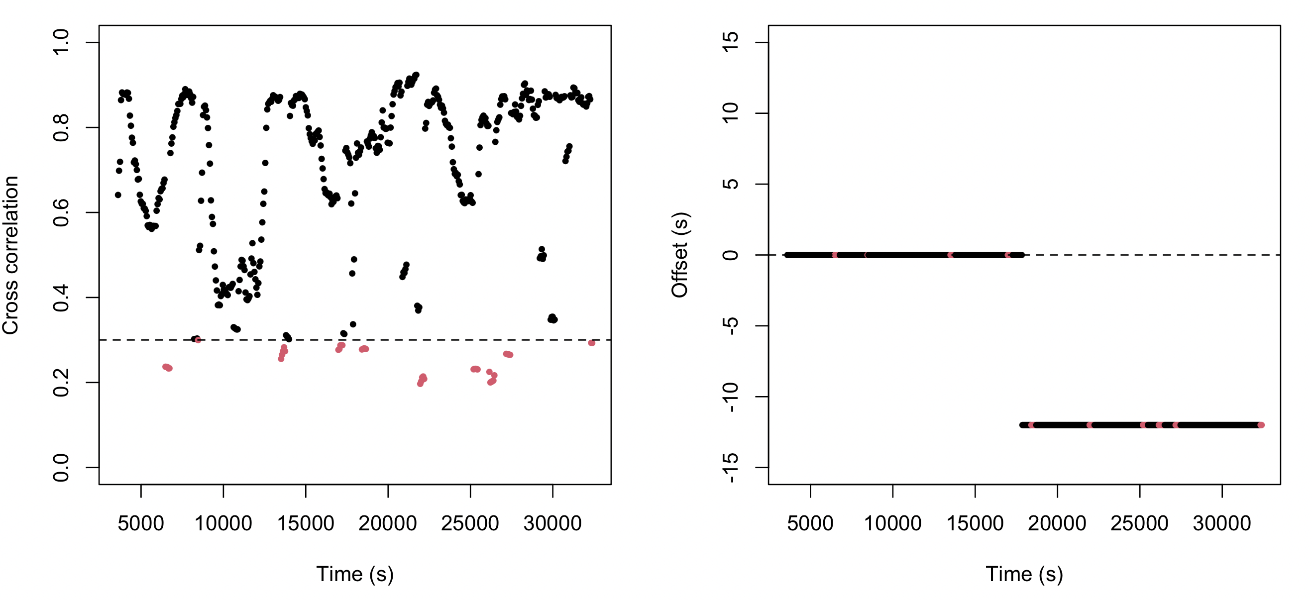
The cross correlations (left panel) look broadly similar (a little more stable, as based on a larger window size - but also exhibiting the same ultradian fluctuation that tracks with sleep stage in this recording). However, the implied pattern of offset across the night is markedly different - a clear step function that corresponds to the 12 second gap that was introduced. Although the slope R2 is still much higher than 0 (i.e. here there is a gap that happens midway through the recording, and so there is a significant change), it very clearly doesn't reflect the type of continuous drift we might expect from miscalibrated clocks.

All the above

What if we put all these things together - can INSERT still yield a clear representation of offset dynamics over the night?

We follow a similar approach as above, first resampling to 200.1 Hz or (as a sanity check) to 199.9 Hz, and saving as text files, i.e.:

luna r-flt.edf -s ' RESAMPLE sr=200.1 & MATRIX file=s201.1.txt min '
luna r-flt.edf -s ' RESAMPLE sr=199.9 & MATRIX file=s199.9.txt min '

We then insert a 12 second interval midway:

awk 'NR==3600000 {for(i=1;i<=2400;i++) print "0"} {print}' s201.1.txt > s201.1_gap.txt
awk 'NR==3600000 {for(i=1;i<=2400;i++) print "0"} {print}' s199.9.txt > s199.9_gap.txt

We then read these back as EDF, but assuming the nominal 200 Hz sample rate; here, also changing the header offset by 42 seconds (i.e. 21.59.19 instead of 22.00.01):

luna s201.1_gap.txt --fs=200 --time=21.59.19 --date=17.07.23 --chs=O1 -s WRITE edf=r-all-fast
luna s199.9_gap.txt --fs=200 --time=21.59.19 --date=17.07.23 --chs=O1 -s WRITE edf=r-all-slow

In summary we have:

• the EDF header time is off by 42 seconds
• one recording has a 12 second gap midway
• one recording has an effective sample rate of 200.1 Hz (or 199.9 Hz) instead of 200 Hz exactly

How does INSERT do? As before, the default run points to low quality alignments, so we run all analyses using shorter windows (len=30):

For the 200.1 Hz example:

  header-derived offset: 42 seconds (negative = edf2 starts after edf1)
  using header-derived offset-range: -18 to 102 seconds
  method: xcorr, bandpass 0.5-15 Hz;  30s windows every 60s,  range 3603-32427s
  summary across 469 window(s):
    quality          accepted=469/481 (97.50%)  peak median=0.79  mean=0.73  min=0.16  max=0.94
    waveform_shift   median=21.03s  mean=15.05s  p10=3.2s  p90=26.7s  min=1.8s  max=28.1s  range=26.3s
    fit_shift        used=469/469  median=21.03s  mean=15.05s  p10=3.2s  p90=26.7s  min=1.8s  max=28.1s  range=26.3s
    offset           47.1782s (start_shift=-5.17818s, header_offset=42s)
    drift            slope=0.0011 s/s  (4.03 s/hr)  intercept=-5.17s  R2=0.906
    implied SR of secondary: 200.225 Hz  (nominal: 200 Hz)
    (positive slope = secondary clock running faster than primary)
  per-pair drift:
    O1..O1:  slope=0.0011s/s (4.038 s/hr)  intercept=-5.17s  implied SR=200.225 Hz

The slope/SR estimate of course confounds the drift and gap together, but visualizing the offset dynamics makes this clearer:

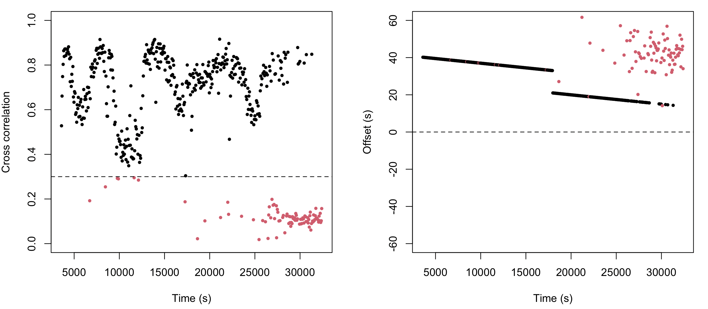
That is, this clearly picks up a) the initial header offset, b) the increased speed (i.e. leading to the lag being reduced) and c) the gap of 12 seconds midway.

And for the 199.9 Hz case:

  header-derived offset: 42 seconds (negative = edf2 starts after edf1)
  using header-derived offset-range: -18 to 102 seconds
  method: xcorr, bandpass 0.5-15 Hz;  30s windows every 60s,  range 3602.3-32420.7s
  summary across 471 window(s):
    quality          accepted=471/481 (97.9%)  peak median=0.79  mean=0.73  min=0.14  max=0.93
    waveform_shift   median=-3.04s  mean=-3.02s  p10=-7.5s  p90=1.55s  min=-8.98s  max=2.99s  range=11.97s
    fit_shift        used=471/471  median=-3.04s  mean=-3.02s  p10=-7.5s  p90=1.55s  min=-8.98s  max=2.99s  range=11.97s
    offset           47.2s (start_shift=-5.22s, header_offset=42s)
    drift            slope=0.00012 s/s  (0.44 s/hr)  intercept=-5.22s  R2=0.104
    implied SR of secondary: 200.025 Hz  (nominal: 200 Hz)
    (positive slope = secondary clock running faster than primary)
  warning: alignment quality may be poor: R2=0.104461 < 0.5
  hints:
    - try a smaller len window (current len=30s)
    - use offset-margin to search around the header-derived offset (current default margin=60s; effective range=-18 to 102s)
    - set an absolute offset-range around the expected shift (current offset-range=unset; effective range=-18 to 102s)
    - use full-search when EDF start times are missing or not trusted (current full-search=no)
    - add verbose=1 to diagnose per-window results (current verbose=no)
  per-pair drift:
    O1..O1:  slope=0.00012 s/s (0.44 s/hr)  intercept=-5.22s  implied SR=200.025 Hz

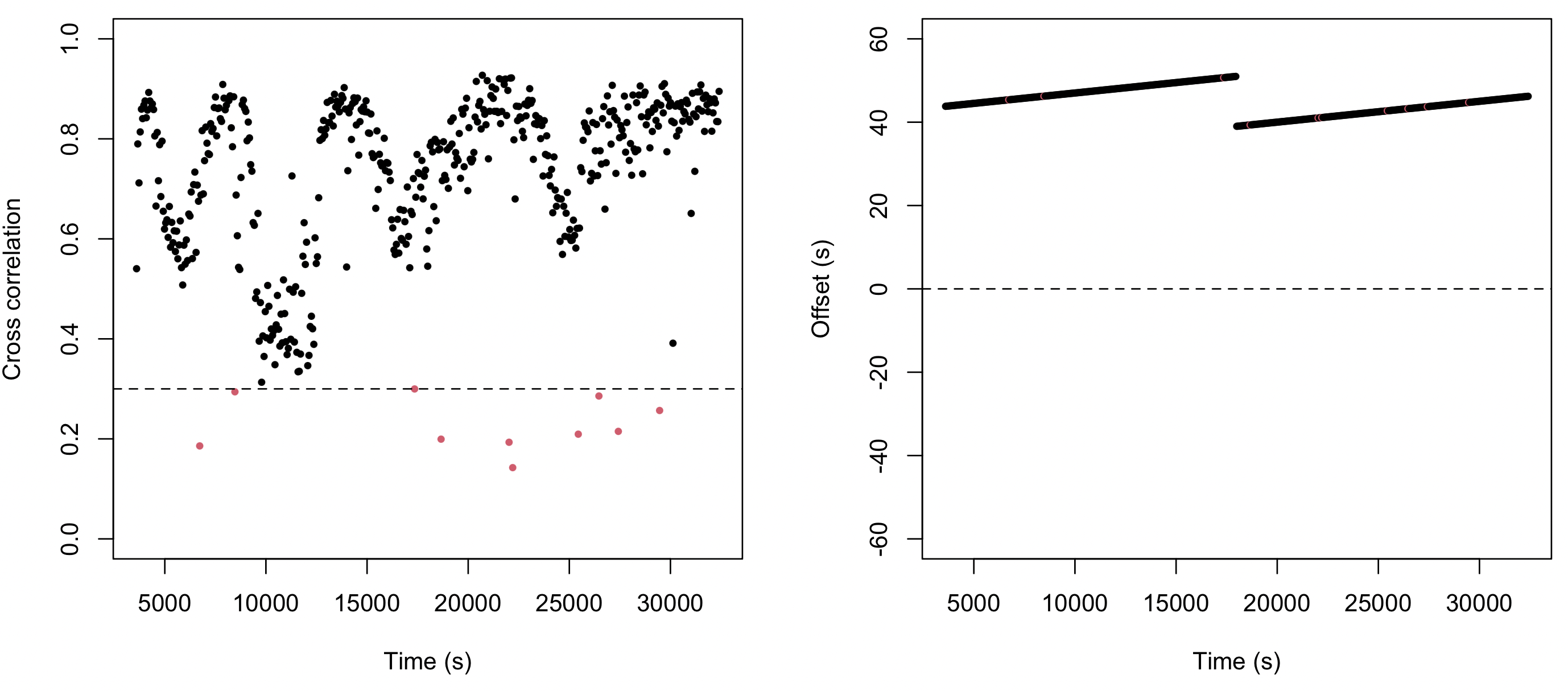
Note the warning stating that the R2 of the drift estimate is very low - meaning we should not trust the implied SR of 200.025 Hz. Again, looking at the plot makes it clear why this is - as the gap and the drift effectively 'cancel out':

Real data example

Now we've oriented ourselves to the INSERT command, we can return to the real-world Nox/X-trodes example.

We'll run this with two pairs of channels: F3 with AF3 and F4 with AF4. This has the advantage of reporting alignment statistics per channel pair, to give a sense of consistency. As these are now genuinely different signals - not just filtered versions of the same signal - we might expect the results to be noisier.

luna nox.edf -o out.db -s ' INSERT edf=xtrodes.edf pairs=F3,AF3,F4,AF4 '

  header-derived offset: -1568 seconds (negative = edf2 starts after edf1)
  using header-derived offset-range: -1628 to -1508 seconds
  method: xcorr, bandpass 0.5-15 Hz;  300s windows every 60s,  range 3220-28980s
  summary across 373 window(s) (22 outlier(s) removed from slope fit):
    quality          accepted=373/430 (86.7%)  peak median=0.45  mean=0.44  min=0.10  max=0.65
    waveform_shift   median=-1594.04s  mean=-1593.7s  p10=-1597.9s  p90=-1589.3s  min=-1608.7s  max=-1582.0s  range=26.6s
    fit_shift        used=351/373  median=-1594.1s  mean=-1593.8s  p10=-1597.7s  p90=-1589.5s  min=-1598.6s  max=-1587.9s  range=10.7s
    offset           31.9038s (start_shift=-1599.9s, header_offset=-1568s)
    drift            slope=0.000412976 s/s  (1.48671 s/hr)  intercept=-1599.9s  R2=0.998
    implied SR of secondary: 200.083 Hz  (nominal: 200 Hz)
    (positive slope = secondary clock running faster than primary)
  per-pair drift:
    F3..AF3:  slope=0.000412 s/s (1.483 s/hr)  intercept=-1599.86s  implied SR=200.082 Hz  [14 outlier(s) removed]
    F4..AF4:  slope=0.000402 s/s (1.449 s/hr)  intercept=-1599.68s  implied SR=200.081 Hz  [24 outlier(s) removed]

Most windows (87%) are accepted as high quality. Here we see an implied drift of around 200.08 Hz, consistent across both channel pairs -- and in fact identical to the estimate we made simply by looking at the two apparent landmarks at the start of this vignette! The R2 for the drift slope is very high (0.998). In addition -- as noted in the plots -- we see an average offset around 30 seconds, suggesting that the EDF headers (which we knew were set at different start times) were also not consistently aligned with each other (i.e. at least one was not using the true clock time). Plotting the results:

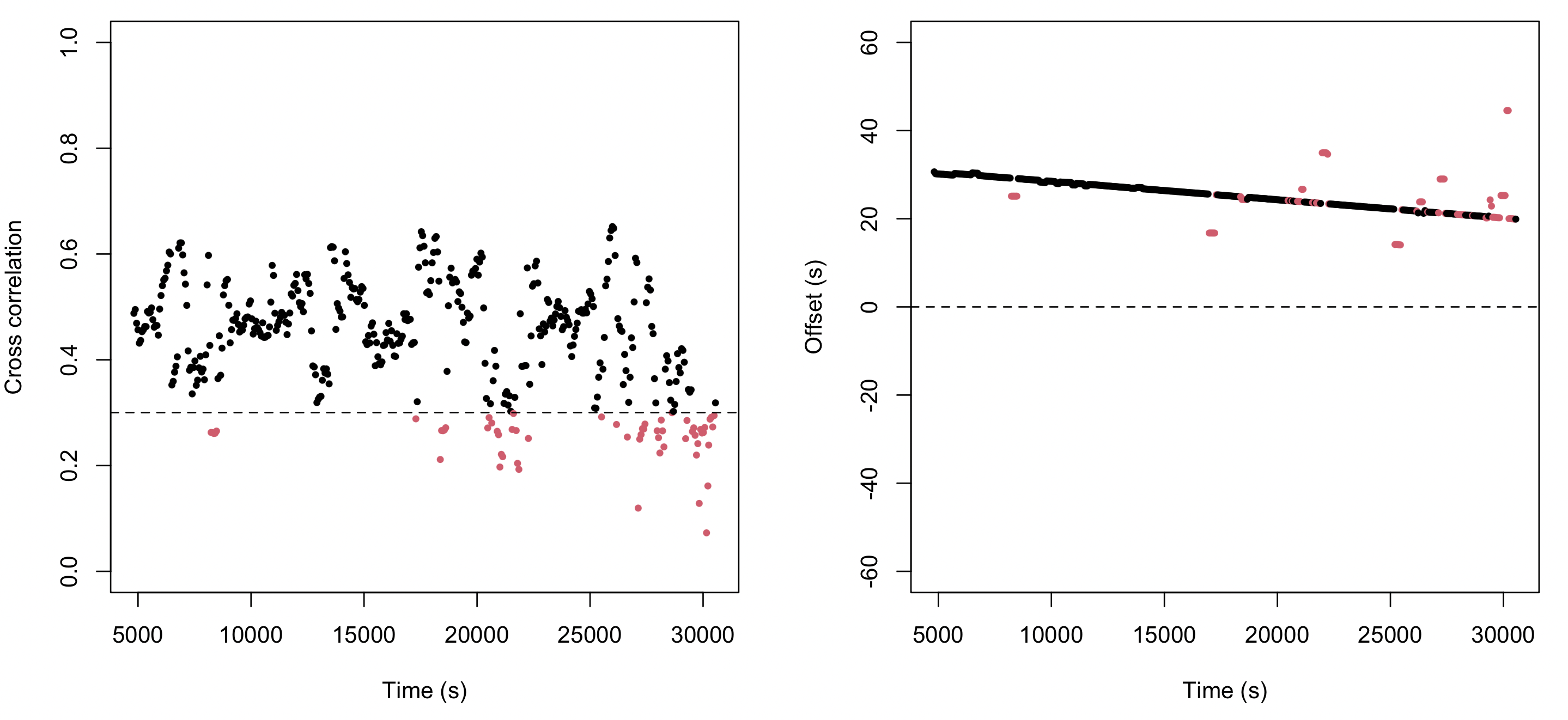
For this recording, the fit was:

• header-derived offset: -1568 s
• median signal-based lag: -1593.94 s
• extra lag beyond the header offset: about 31 s early in the night and 23 s near 04:26
• fitted drift: 0.000413 s/s, or 1.487 s/hr
• implied X-trodes sample rate after correction: 200.083 Hz
• accepted windows: 373/430 with R2=0.998

The point is not only that there is a start offset, but that the residual offset changes across the night. Even after accounting for the EDF start times, the two clocks keep sliding relative to each other.

Fixing the alignment

Once the offset and drift have been estimated, the actual corrected insert is straightforward:

luna nox.edf -s ' INSERT edf=xtrodes.edf pairs=F3,AF3,F4,AF4 insert & WRITE edf=aligned '

That is: we add the insert option and then WRITE out a new EDF, which will have the new signals included.

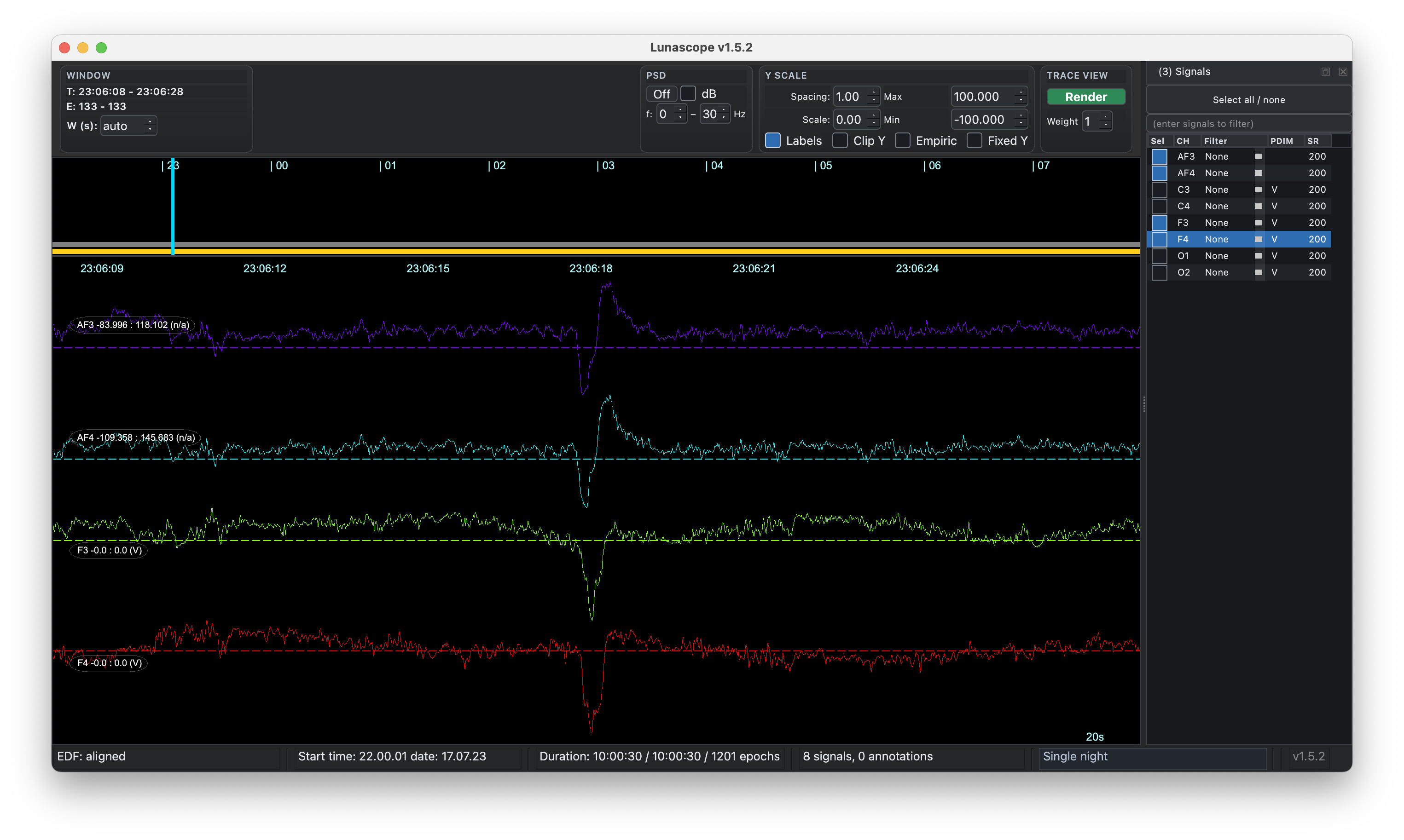
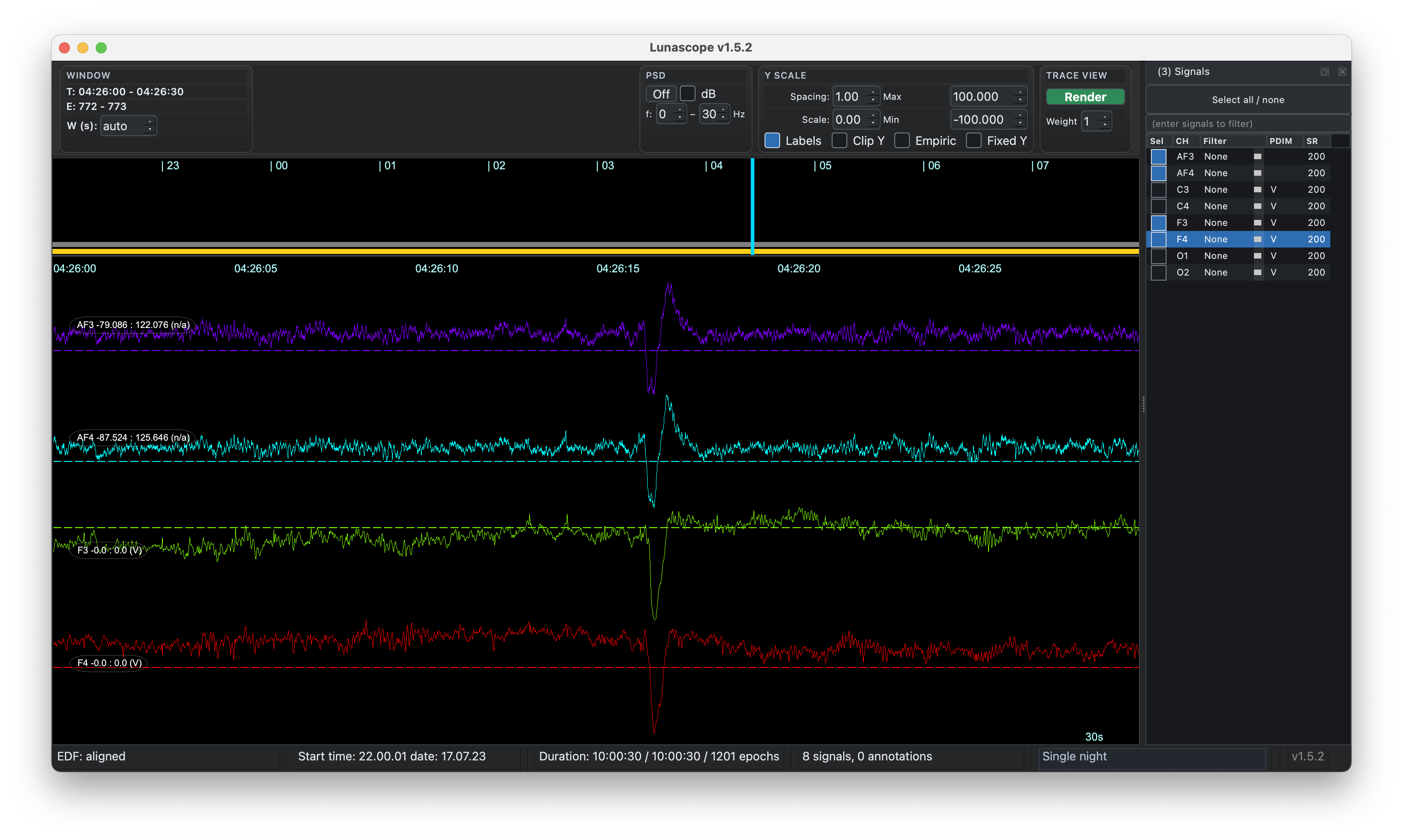
We can now look at aligned.edf in Lunascope, revisiting the two visually clear misalignments shown above. Both regions are now very closely aligned:

This is the real utility of INSERT: not simply to merge EDFs, but to make long, multi-sensor recordings meaningfully comparable on a common timeline.

Inserting new signals

It is also possible to specify the offset (and drift) explicitly rather than estimate them from data (i.e. this may be possible if other sources of time-marking exist). In this case, we can do a direct merge (as used to make the EDF for the original plots at the top of this vignette):

luna nox.edf -s ' INSERT edf=xtrodes.edf offset=-1568 & WRITE edf=merged '

Note that although the sampling rates of signals used by pairs must be similar, in general, INSERT can insert signals of any sampling rate - i.e. in the original plots of merged.edf, the X-trodes signals had very high sampling rates (4000 Hz). If one wanted to retain that in aligned.edf, then based on the empirical cross-correlation analyses one could duplicate those samples in the EDF, resampling one set to use for alignment.

Importantly, the "fix" presented here only corrects for a) an offset/intercept and b) a linear slope. It does this via cubic spline interpolation when making the new signals, appropriately time-stretching drifting signals. In contrast, it cannot handle gaps/jumps or other non-linear types of effect. In those cases, reviewing the discontinuities from the plots as above, splitting the recordings, and doing piecewise correction would be the solution: INSERT could be used in that scenario, but not in a single, automated manner.

Sensitivity analyses

Choice of alignment pairs matters. More similar sensors give cleaner cross-correlation peaks and a more stable fit. In this example we compared F3/F4 to the wearable frontal channels, with good results. What if we instead used the two central channels, or even the two occipital Nox channels (e.g. if those were all we had). (Note: you can specify that one channel is paired with multiple others as needed, e.g. if we only had Fz in the Nox recording, we could use pairs=Fz,AF3,Fz,AF4.)

Re-running with pairs=C3,AF3,C4,AF4 gives:

  header-derived offset: -1568 seconds (negative = edf2 starts after edf1)
  using header-derived offset-range: -1628 to -1508 seconds
  method: xcorr, bandpass 0.5-15 Hz;  300s windows every 60s,  range 3220-28980s
  summary across 242 window(s) (13 outlier(s) removed from slope fit):
    quality          accepted=242/430 (56.2791%)  peak median=0.315217  mean=0.310662  min=0.0709152  max=0.694037
    waveform_shift   median=-1594.52s  mean=-1594.41s  p10=-1598.5s  p90=-1589.2s  min=-1618.39s  max=-1582.12s  range=36.28s
    fit_shift        used=229/242  median=-1594.46s  mean=-1594.17s  p10=-1598.09s  p90=-1589.71s  min=-1604.95s  max=-1586.45s  range=18.5s
    offset           31.9633s (start_shift=-1599.96s, header_offset=-1568s)
    drift            slope=0.000402523 s/s  (1.44908 s/hr)  intercept=-1599.96s  R2=0.699277
    implied SR of secondary: 200.081 Hz  (nominal: 200 Hz)
    (positive slope = secondary clock running faster than primary)
  warning: alignment quality may be poor: median peak=0.315217 < 0.35
  hints:
    - try a smaller len window (current len=300s)
    - use offset-margin to search around the header-derived offset (current default margin=60s; effective range=-1628 to -1508s)
    - set an absolute offset-range around the expected shift (current offset-range=unset; effective range=-1628 to -1508s)
    - use full-search when EDF start times are missing or not trusted (current full-search=no)
    - add verbose=1 to diagnose per-window results (current verbose=no)
  per-pair drift:
    C3..AF3:  slope=0.000415154 s/s (1.49455 s/hr)  intercept=-1599.91s  implied SR=200.083 Hz  [23 outlier(s) removed]
    C4..AF4:  slope=0.000529584 s/s (1.9065 s/hr)  intercept=-1600.78s  implied SR=200.106 Hz  [8 outlier(s) removed]

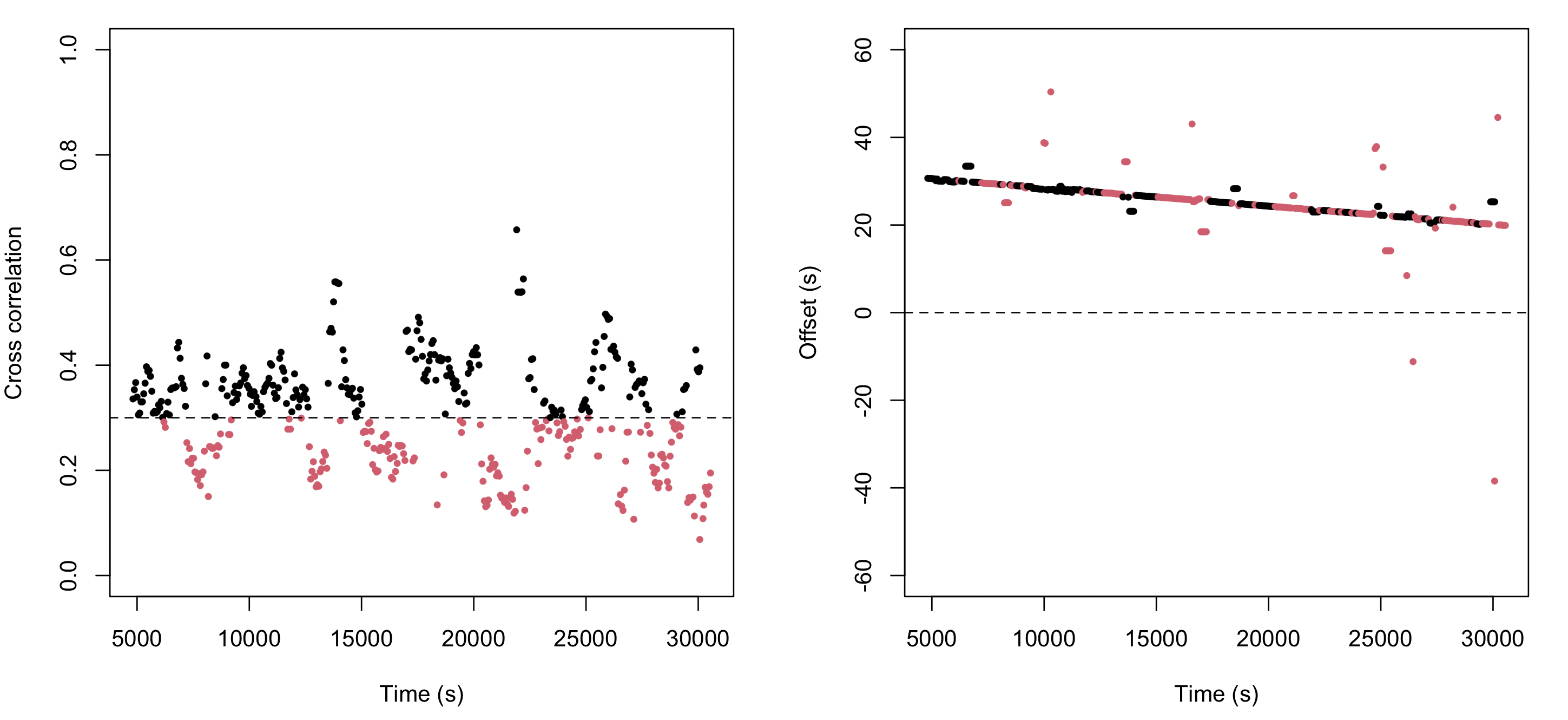
Only 56% of windows are deemed to be good here, which is worse than the frontal case. We'll skip it here, but you can alter the parameters in search of a better fit: the auto-try command and its variants can be helpful by scanning across different parameter values. Here we see that shorter windows (but longer than 30s) may be helpful:

    start=3220s len=30s inc=6s  accepted=3232/4294  P_OK=0.752678  peak=0.365709  R2=0.27623   score=0.076035
    start=3220s len=75s inc=15s  accepted=1172/1718  P_OK=0.682189  peak=0.34891  R2=0.959133  score=0.228295
    start=3220s len=150s inc=30s  accepted=544/859  P_OK=0.633295  peak=0.334924  R2=0.951135  score=0.201741
    start=3220s len=300s inc=60s  accepted=242/430  P_OK=0.562791  peak=0.315217  R2=0.699277  score=0.124053

For the occipital channels, as expected, the ability to align studies diminishes - but not completely:

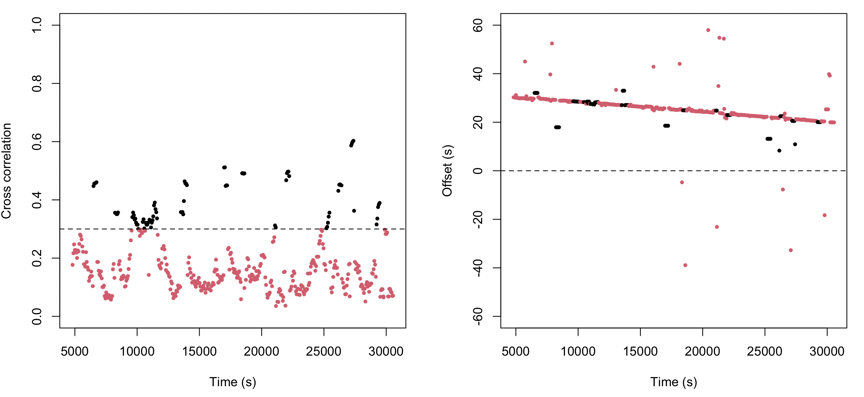
Even here, altering parameters can increase the consistency of the estimates under a linear-drift model (i.e. high R2) while retaining a sufficiently large number of windows. Running with:

  fit-outlier-passes=4 fit-outlier-sd=2 len=60 min-peak=0.2

gives R2=0.99 based on 231 windows.

Overall, the ranking is exactly what we would expect: frontal performed best, central was usable but clearly weaker, and occipital was poor.

• Frontal (F3/F4 vs AF3/AF4) was the strongest run: high acceptance (373/430, 87%), the best median peak (0.45), and an excellent drift fit (R2=0.998). The implied SR was also very consistent at about 200.083 Hz, and the two pairwise slopes matched closely.

• Central (C3/C4 vs AF3/AF4) degraded substantially: acceptance dropped to 56%, median peak fell to 0.32, and R2 dropped to 0.7, enough to trigger the low-peak warning. The overall offset/drift estimate stayed in the same ballpark, but the fit was clearly less stable and the pairwise SR estimates spread more.

• Occipital (O1/O2 vs AF3/AF4) was weak enough to be unreliable: under default parameter settings, only 20% of windows were accepted, median peak was just 0.15, and R2 fell to 0.42, with warnings on all three quality criteria. Nonetheless, the offset estimate still landed near the same value, and changing parameter settings improved performance.

Even for the occipital case, visual review of the offset over time was strongly suggestive of the same drift that we saw for the other channels - this alone is sufficient to suggest that we are still picking up information relevant to assessing drift from this comparison. This is in large part because the most informative features may be movement artifacts and so on that are shared between channels. Ironically, this means that noisier data may be easier to fix, if there are timing issues. The extent to which other types of signals (e.g. ECG, EMG) can be used is an open question - but one that can be approached empirically, using the type of simulations as above.

Parameter tuning

For modest offsets and drift, the defaults are often fine. If the signals differ a lot, or the clocks are substantially off, it helps to try a range of settings:

• pairs=: the most important choice. Use the most similar channels you can.
• offset-margin=: when EDF header times are roughly right, search around that implied offset (default +/-60s).
• offset-range=: use this when the header is unreliable and you need a wider absolute search window.
• len=: shorter windows (e.g. 30s) can tolerate larger local drift (default 300s); longer windows can sharpen the xcorr peak when the mismatch is small.
• start=: skipping the start of the file can avoid unstable initial segments.
• min-peak=: lower from the default of 0.3 to allow a greater number of low-quality windows, but then you may want to compensate with more stringent outlier detection at the linear fit stage.
• fit-outlier-sd=: decrease (from 3) to be more stringent in excluding windows at the linear fit stage.
• fit-outlier-passes=: increase (from 2) to be more stringent in excluding windows at the linear fit stage.
• inc=: smaller increments give more windows and a denser fit, at the cost of more computation.
• full-search: if clocks are very miscalibrated (e.g. off by many minutes, hours) this can be useful: it is much slower, so increase inc to reduce the number of windows; also run with verbose=1 to see the window-by-window alignments more clearly.
• auto-try: useful when you expect that one fixed start/len/inc choice may not be optimal.

In general, if the offset is large, begin by broadening offset-margin or offset-range; if the xcorr peaks are smeared by drift, shorten len; if the fit is unstable, try more similar channels, move start away from noisy leading segments, or let auto-try search a local grid. If still not aligning, try full-search. Remember, it is also useful to view e.g. EEG spectrograms for both studies, to assess by eye whether these look like the same night with similar ultradian structure and sufficiently high-quality signals.

Conclusion

INSERT is most useful when two recordings are clearly related but do not share a trustworthy timeline. In the examples above, it distinguishes simple header offsets from continuous drift and from discrete gaps, and it shows when a single linear correction is likely to be valid. In practice, the workflow is straightforward: choose the most comparable channel pairs, inspect the quality metrics and offset-by-time plots, and then apply the empirical correction only when the fit is coherent. It is crucially important to inspect the diagnostic outputs: do not try to run this command blindly and expect magic to happen...

The key limitation is also clear from these examples: INSERT can correct a start offset and linear drift, but it does not by itself resolve non-linear timing problems such as gaps or jumps. When those are present, the diagnostic plots are still informative, but correction needs to be done in pieces rather than through one automatic alignment step.